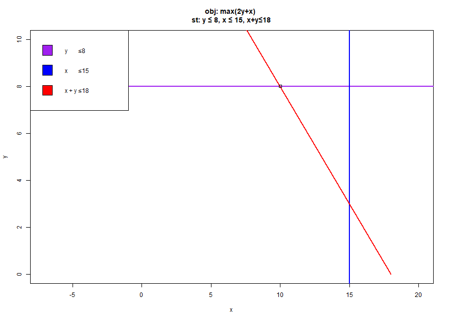
Linear programming

Linear programming (LP) is a method to provide an optimal solution to a problem defined by a set of linear constraints. It is very widely applied in engineering and science.

A typical linear programming problem is defined by an Objective function (the target to maximise or minimise) and a set of constraints which limit the solution space.

What does an LP problem look like?

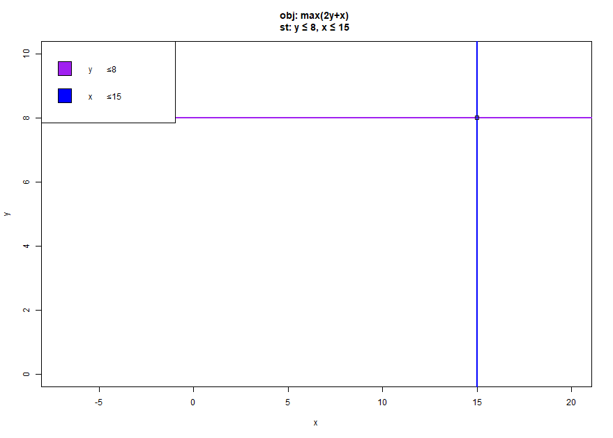
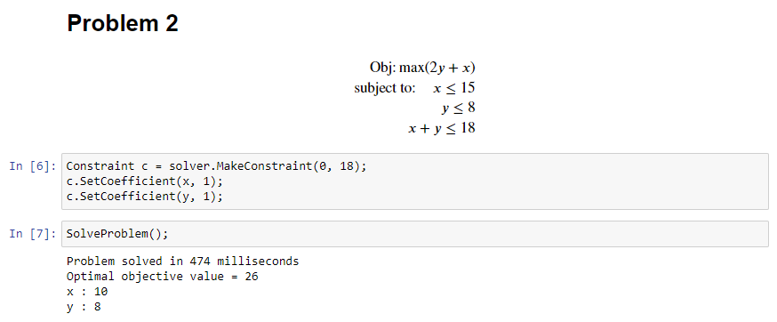
We are going to start with a very simple linear problem definition. The first line of the problem describes the objective function, in this the value to maximize. In this problem, we have two variables to optimize x and y. The constraints that limit the problem's space are defined under the subject to section.

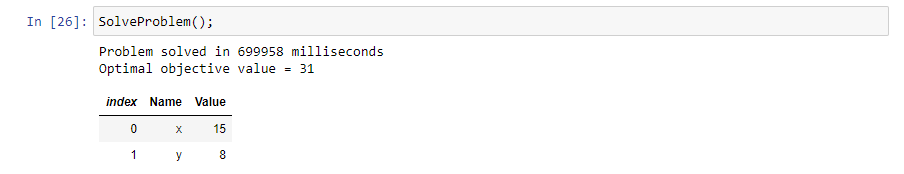
This very simple maximisation problem has a maximum solution of \(x=15\) and \(y=8\) for an objective value of \(31\) .

There exist many linear programming solvers to calculate this optimum. We will be using Coin-OR project CLP with the Google OR-Tools as an interface for C#.

Meet the solver

You can find my notebook with all the code here. And you can now access the Jupyter notebooks online, thanks to Binder!

Coin-OR¹ CLP (with Google OR¹-Tools)

The Coin-OR project provides high quality solvers for many applications with an open source license. CLP is the main linear programming solver we will be using until we start adding binary variables, at which point we will start using CBC. To call them from C#, we could write out a format that CLP / CBC knows how to read, such as MPS or we could use a wrapping library to call them directly from C#. We will be focusing on using the Google OR-Tools.

Google OR-Tools

The Google OR-Tools provide us with a set of primitives with which to work with so that we can define optimisation problems and allow us to call to various solvers, including CLP, which we will be using. Also the OR-Tools provide routines to write out the problems in MPS and other formats. We will focus on using the OR Tools as soon as the introduction is over.

Adding the Google OR Tools through nuget to the Jupyter notebook with the #r command and using in the cell imports the solver.

#r "nuget:Google.OrTools"

using Google.OrTools.LinearSolver;

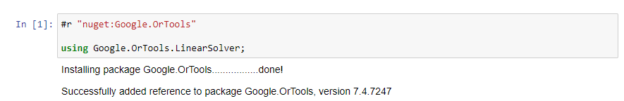
This allows us to create a solver instance as follows, note the constant CLP_LINEAR_PROGRAMMING this tells us which solver we will be using.

Solver solver = Solver.CreateSolver("LinearProgramming", "CLP_LINEAR_PROGRAMMING");

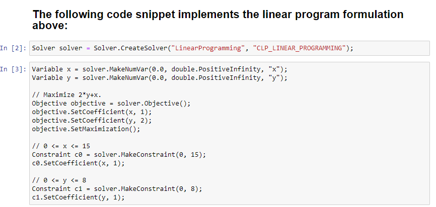
The following code snippet implements the linear program formulation below²:

The solver has been already defined and initalized. We are now defining the variables of the problem, the objective function and the linear constraints that apply.

Variable x = solver.MakeNumVar(0.0, double.PositiveInfinity, "x");
Variable y = solver.MakeNumVar(0.0, double.PositiveInfinity, "y");

// Maximize 2*y+x.
Objective objective = solver.Objective();
objective.SetCoefficient(x, 1);
objective.SetCoefficient(y, 2);
objective.SetMaximization();

// 0 <= x <= 15 
Constraint c0 = solver.MakeConstraint(0, 15);
c0.SetCoefficient(x, 1);

// 0 <= y <= 8
Constraint c1 = solver.MakeConstraint(0, 8);
c1.SetCoefficient(y, 1);

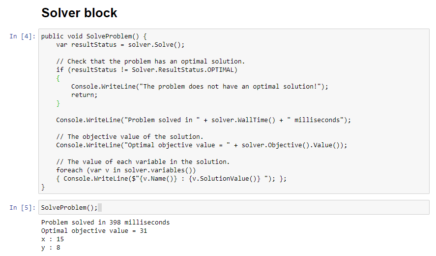
When you execute the next cells, the solver.Solve() function is called and the results will be written out to the cell's output. We will use this function cell several times over the course of the workbook.

public void SolveProblem() {
    var resultStatus = solver.Solve();

    // Check that the problem has an optimal solution.
    if (resultStatus != Solver.ResultStatus.OPTIMAL)
    {
        Console.WriteLine("The problem does not have an optimal solution!");
        return;
    }

    Console.WriteLine("Problem solved in " + solver.WallTime() + " milliseconds");

    // The objective value of the solution.
    Console.WriteLine("Optimal objective value = " + solver.Objective().Value());

    // The value of each variable in the solution.
    foreach (var v in solver.variables())
    { Console.WriteLine($"{v.Name()} : {v.SolutionValue()} "); };
}

Other solvers

There exists many other solvers that are available, either directly wrapped through the Google OR Tools such as GLOP or another library or as external programs fed through input files in MPS or other formats. The NEOS project provides a thorough set of optimisation solvers that are available online with many input formats available (MPS, AMPL, Lp, GAMS).

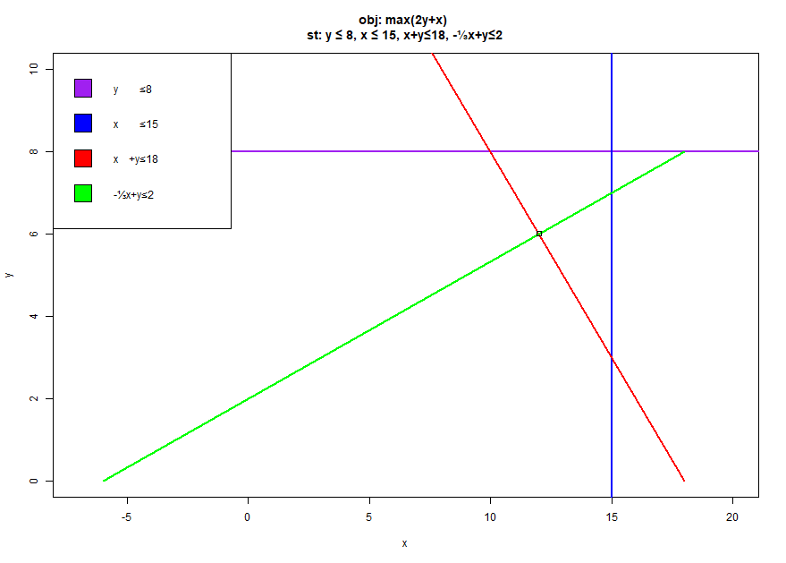
Problem 2

We will be adding a third constraint to the formulation of Problem 1.

The solver is initialized with the full problem 1 defintion already, x and y are already declared. When you click run on the solver's cell, the solver.Solve() function is called and results are written out.

Constraint c = solver.MakeConstraint(0, 18);
c.SetCoefficient(x, 1);
c.SetCoefficient(y, 1);

If you call SolveProblem();, you will now have a new optimal value that is lower that the previous one. In linear programming maximization problem, adding a new constraint will always make the optimal value lower or equal to the less constrained. problem

Problem 3

You should now be able to add an adding a fourth constraint to the formulation of Problem 2.

The solver is initialized with the full problem 2 defintion already, x and y are already declared. When you click on the solver's cell, the solver.Solve() function is called and results are written out.

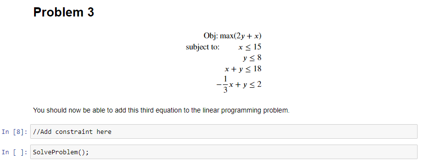
For those following along in the notebook there is a hint below this section with a second implementation of the SolveProblem() function which should give you hints based on your objective value.

The power of Jupyter special commands

I'm discovering slowly the jupyter commands. The first command display() allows you to present objects in a table. A great way to select the properties you want to show is to use linq (remember to add using System.Linq) to map a list of objects to an anonymous object with the properties you want to show in the table.

display(solver.variables().Select(a => new { Name  = a.Name(), Value = a.SolutionValue() }));

Recap

Now that we have introduced linear programming and know how to use the solver, the following chapter will cover two simple linear programming applications.